결측치의 처리

impute

Author

강신성

Published

2023-10-19

결측치를 시각화해보고, 계산해서 대치(impute)해보기도 하자!

해당 포스트는 전북대학교 통계학과 최규빈 교수님의 강의내용을 토대로 재구성되었음을 알립니다.

1. 라이브러리 imports

#!pip install missingno # missingno 라이브러리가 설치되어있지 않을 경우

import pandas as pd
import numpy as np
import missingno as msno
import sklearn.impute

2. `missingno`의 활용

df = pd.read_csv("https://raw.githubusercontent.com/guebin/MP2023/main/posts/msno.csv")
df

	A	B	C	D	E
0	0.383420	1.385096	NaN	-0.545132	-0.732395
1	1.084175	0.080613	-0.770527	-0.272143	-0.749881
2	1.142778	1.258419	NaN	-0.072007	-0.440757
3	0.307894	0.521400	0.446974	0.329530	-1.457388
4	0.237787	0.132401	-0.516630	0.177995	0.416182
...	...	...	...	...	...
995	0.041092	-1.308165	1.085820	1.136210	NaN
996	-1.286358	1.547987	NaN	-0.174334	-0.579486
997	0.710257	1.764058	NaN	-0.353928	NaN
998	-1.908729	-0.804691	NaN	NaN	-0.066739
999	0.650026	2.206549	NaN	-0.919945	NaN

1000 rows × 5 columns

결측치가 딱봐도 엄청 많아보인다. missingno는 그것을 시각화해준다.

msno.matrix(df)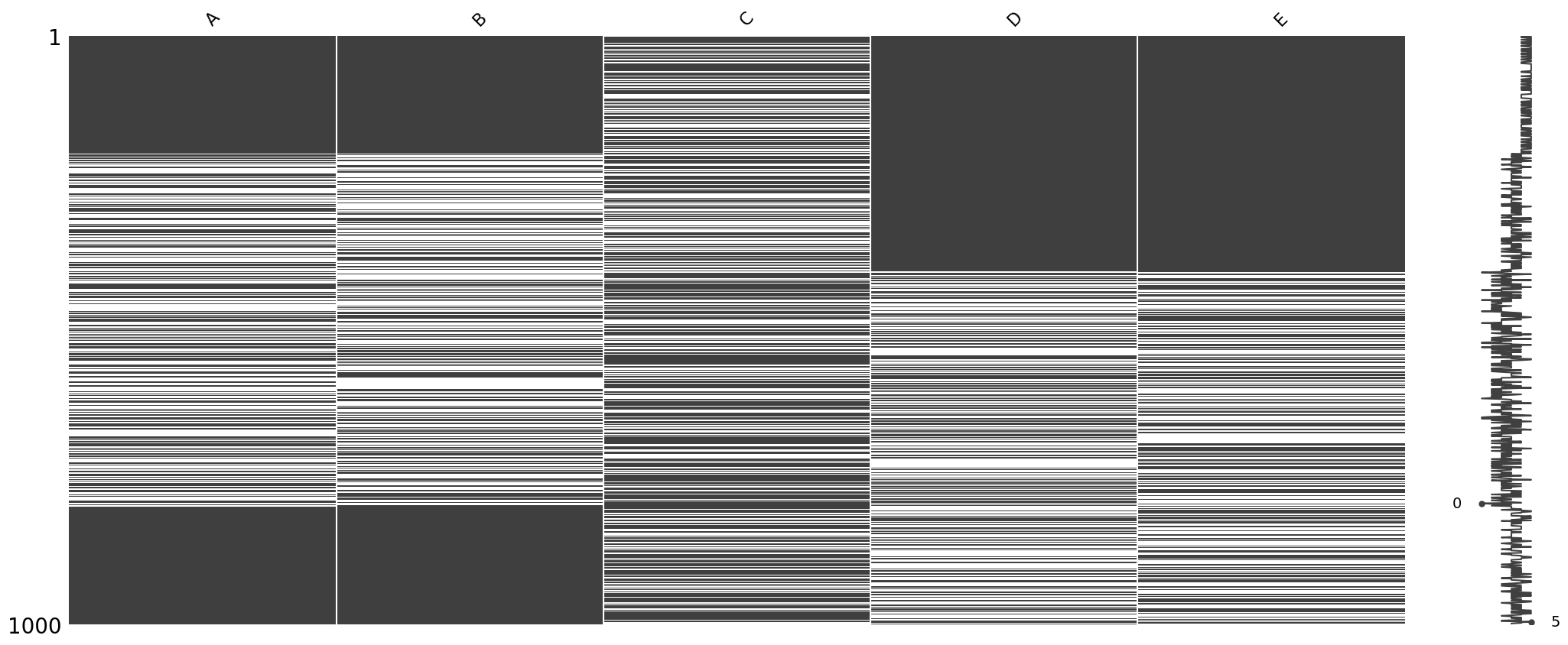

우측 노이즈와 같은 그래프에서 0에 있는 것은 해당 행에 데이터가 하나도 없다는 뜻이고, 5에 있는 것은 다섯개의 데이터가 해당 행에 존재한다는 것이다. 데이터셋이 다섯개니까 그 합이 그래프로 표기된다.

msno.heatmap(df)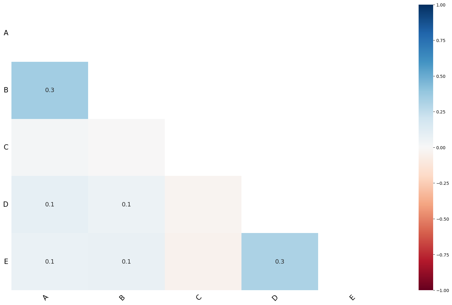

msno.dendrogram(df)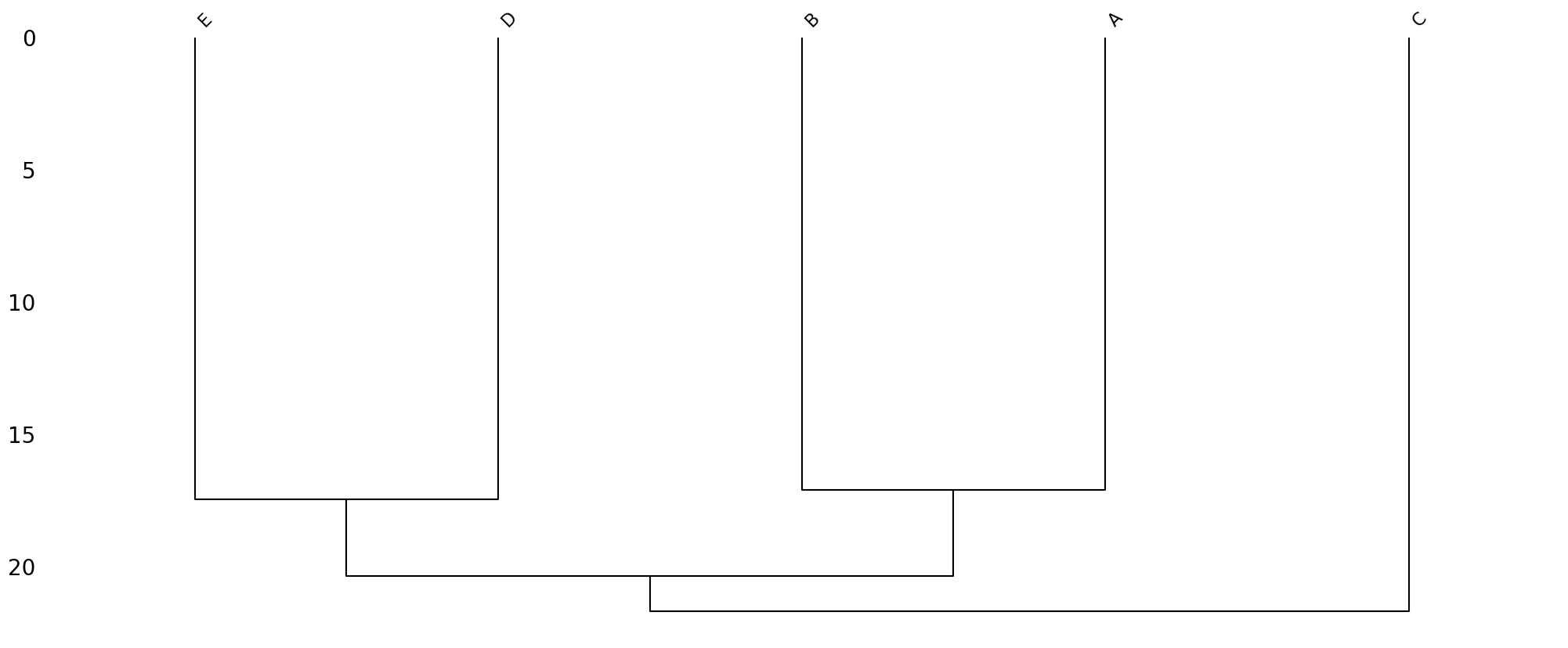

구조가 비슷한 자료들을 엮어놓는다.

그럼 시각화를 했으니까, 이제 결측치를 처리해야겠지?

3. 숫자형 자료의 impute(결측치를 대체하는 것)

- 주어진 자료

A = [2.1, 1.9, 2.2, np.nan, 1.9]
B = [0, 0, np.nan, 0, 0]

df = pd.DataFrame({'A' : A, 'B' : B})
df

	A	B
0	2.1	0.0
1	1.9	0.0
2	2.2	NaN
3	NaN	0.0
4	1.9	0.0

결측치를 무엇으로 채워주면 좋을까?

일단 평균으로 해보면 얼추 맞을 것 같다.

df2 = df
df2.loc[3, 'A'] = df2.A.mean()  ## mean과 같은 메소드는 결측치를 반영하지 않는다.
df2.loc[2, 'B'] = df2.B.mean()
df2

	A	B
0	2.100	0.0
1	1.900	0.0
2	2.200	0.0
3	2.025	0.0
4	1.900	0.0

- 근데 이게 엄청 많으면 언제 다 일일히 하고 있어? > 자동으로 하려면?

(방법1) | 평균으로 impute

imputr = sklearn.impute.SimpleImputer()  ## SimpleImputer(strategy = 'mean')
imputr

SimpleImputer()

In a Jupyter environment, please rerun this cell to show the HTML representation or trust the notebook.
On GitHub, the HTML representation is unable to render, please try loading this page with nbviewer.org.

predictr.fit하는 것처럼 결측치가 있는 열에 적합해야 한다.

imputr.fit(df)

SimpleImputer()

predictr.predict하는 것처럼 인풋시켜야 한다.

imputr.transform(df)

array([[2.1  , 0.   ],
       [1.9  , 0.   ],
       [2.2  , 0.   ],
       [2.025, 0.   ],
       [1.9  , 0.   ]])

위에서와 똑같은 결과를 산출했다.

해당 과정은 imputr.fit_transform(df)로 한번에 시행할 수 있다.

- 만약 평균이 아닌 다른 방식으로 결측치를 대체하고 싶다면…

(방법 2) | median으로 impute

imputr = sklearn.impute.SimpleImputer(strategy = 'median')
imputr.fit_transform(df)

array([[2.1  , 0.   ],
       [1.9  , 0.   ],
       [2.2  , 0.   ],
       [2.025, 0.   ],
       [1.9  , 0.   ]])

(방법 3) | 최빈값으로 대체

imputr = sklearn.impute.SimpleImputer(strategy = 'most_frequent')
imputr.fit_transform(df)

array([[2.1  , 0.   ],
       [1.9  , 0.   ],
       [2.2  , 0.   ],
       [2.025, 0.   ],
       [1.9  , 0.   ]])

(방법 4) | 정해진 상수값으로 대체

imputr = sklearn.impute.SimpleImputer(strategy = 'constant', fill_value = 999)
imputr.fit_transform(df)

array([[2.1  , 0.   ],
       [1.9  , 0.   ],
       [2.2  , 0.   ],
       [2.025, 0.   ],
       [1.9  , 0.   ]])

4. 범주형 자료의 impute

df = pd.DataFrame({'A':['Y','N','Y','Y',np.nan], 'B':['stat','math',np.nan,'stat','bio']})
df

	A	B
0	Y	stat
1	N	math
2	Y	NaN
3	Y	stat
4	NaN	bio

(방법 1) | 최빈값을 이용

imputr = sklearn.impute.SimpleImputer(strategy = 'most_frequent')
imputr.fit_transform(df)

array([['Y', 'stat'],
       ['N', 'math'],
       ['Y', 'stat'],
       ['Y', 'stat'],
       ['Y', 'bio']], dtype=object)

(방법 2) | 상수(지정값)로 대체함

imputr = sklearn.impute.SimpleImputer(strategy = 'constant', fill_value = 'G')
A_ = pd.Series(imputr.fit_transform(df[['A']]).reshape(-1))
imputr = sklearn.impute.SimpleImputer(strategy = 'constant', fill_value = 'economy')
B_ = pd.Series(imputr.fit_transform(df[['B']]).reshape(-1))

pd.concat([A_, B_], axis = 1).set_axis(['A','B'], axis = 1)

	A	B
0	Y	stat
1	N	math
2	Y	economy
3	Y	stat
4	G	bio

## 또는
imputr = sklearn.impute.SimpleImputer(strategy = 'constant', fill_value = 'G')
A_ = imputr.fit_transform(df[['A']])
imputr = sklearn.impute.SimpleImputer(strategy = 'constant', fill_value = 'economy')
B_ = imputr.fit_transform(df[['B']])

pd.DataFrame(np.concatenate([A_,B_], axis = 1), columns = ['A','B'])

	A	B
0	Y	stat
1	N	math
2	Y	economy
3	Y	stat
4	G	bio

일반적으로 연속형ㆍ숫자형 자료에는 평균, 범주형 자료에는 최빈값으로 대체한다.

해당 포스트는 전북대학교 통계학과 최규빈 교수님의 강의내용을 토대로 재구성되었음을 알립니다.

1. 라이브러리 imports

2. missingno의 활용

3. 숫자형 자료의 impute(결측치를 대체하는 것)

4. 범주형 자료의 impute

2. `missingno`의 활용